Lesson 2: Entering Text

In this lesson you are going to learn how to enter text.  To begin, open Microsoft Excel. For this lesson, your default font should be set to Arial. Let�s check to make sure it is.

1. Click on Format, which is located on the Menu bar.
2. Press the down arrow key until Style is highlighted.
3. Press Enter. A dialog box will appear.
4. Click on Modify.
5. Click on the Font tab, if it is not in the front.
6. Click on Arial in the Font box, if Arial is not already selected.
7. Click on OK.
8. Click again on OK.

1. Place the cursor in cell A1.
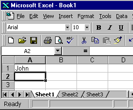
2. Type John Jordan. Note that the word Ready on the Status bar changes to Enter.
3. The Backspace key erases one character at a time. Erase "Jordan" by pressing the backspace key until Jordan is erased.
4. Press Enter. The name "John" should appear in cell A1.

Editing a Cell

After you enter data into a cell, you can edit it by pressing F2 while you are in the cell you wish to edit.

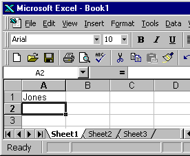
1. Move the cursor to cell A1.
2. Press F2. Note that the word Ready on the Status bar changes to Edit.
3. Change "John" to "Jones."
4. Use the backspace key to delete the "n" and the "h."
5. Type nes.
6. Press Enter.

Alternate Method � Editing a Cell by Using the Formula Bar

You can also edit the cell by using the Formula bar. You can change "Jones" to "Joker" as follows:

1. Move the cursor to cell A1.
2. Click in the formula area of the Formula bar.

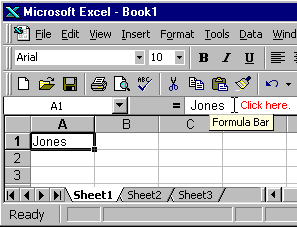
3. Use the backspace key to erase the "s," "e," and "n."
4. Type ker.
5. Press Enter.

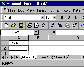
Alternate Method � Editing a Cell by Double-Clicking in the Cell

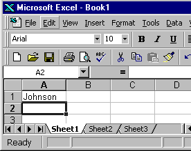
You can change "Joker" to "Johnson" as follows:

1. Move the cursor to cell A1.
2. Double-click in cell A1.
3. Press the End key. That will place the cursor at the end of your text.
4. Use the backspace to erase "r," "e," and "k."
5. Type hnson.
6. Press Enter.

Changing a Cell Entry

Typing in a cell while you are in the Ready mode will replace the old cell entry with the new information you type.

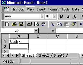
1. Move the cursor to cell A1.
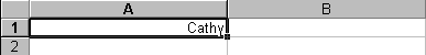
2. Type Cathy.
3. Press Enter. The name "Cathy" should replace "Johnson."

Adjusting the Standard Column Width

When you enter Microsoft Excel, the width of each cell is set to a default width. This width is called the standard column width. We need to change the standard column width to complete our exercises. To make the change, follow these steps:

1. Click on Format, which is located on the Menu bar.
2. Press the down arrow key until Column is highlighted.
3. Press Enter.
4. Press the down arrow key until Standard Width is highlighted.
5. Press Enter.
6. Type 25 in the Standard Column Width field.
7. Click on OK. The width of every cell on the worksheet should now be set to 25.

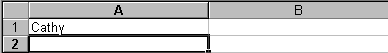
Look at cell A1. The name "Cathy" is aligned with the left side of the cell. You can change the cell alignment.

Centering by Using the Menu

To center the name Cathy, follow these steps:

1. Move the cursor to cell A1.
2. Click on Format, which is located on the Menu bar.
3. Press the down arrow key until Cells is highlighted.
4. Press Enter.
5. Click on the Alignment tab, if it is not in the front.
6. Click to open the drop-down box associated with the Horizontal field. After the drop-down box is opened, click on Center.
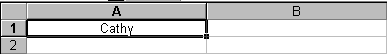
7. Click on OK to close the dialog box. The name "Cathy" should now be centered.

Right-Aligning by Using the Menu

To right-align the name "Cathy," follow these steps:

1. Move the cursor to cell A1.
2. Click on Format, which is located on the Menu bar.
3. Press the down arrow key until Cells is highlighted.
4. Press Enter.
5. Click on the Alignment tab, if it is not in the front.
6. Click to open the drop-down box associated with the Horizontal field. After the drop-down box is opened, click on Right.
7. Click on OK to close the dialog box. The name "Cathy" should now be right-aligned.

Left-Aligning by Using the Menu

To left-align the name "Cathy," follow these steps:

1. Move the cursor to cell A1.
2. Click on Format, which is located on the Menu bar.
3. Press the down arrow key until Cells is highlighted.
4. Press Enter.
5. Click on the alignment tab, if it is not in the front.
6. Click to open the drop-down box associated with the Horizontal field. After the drop-down box is opened, click on Left (Indent).
7. Click on OK to close the dialog box. The name "Cathy" should now be left-aligned.

Alternate Method -- Alignment by Using the Formatting Toolbar

Using the Formatting toolbar, you can quickly perform functions. You can use the Formatting toolbar to change alignment.

Centering by Using the Toolbar

To center the name "Cathy," follow these steps:

1. Move the cursor to cell A1.
2. Click on the Center icon, which is located on the Formatting toolbar.

The red circle designates the Align Center icon.

Right-Aligning by Using the Toolbar

To right-align the name "Cathy," follow these steps:

1. Move the cursor to cell A1.
2. Click on the Align Right icon, which is located on the Formatting toolbar.

The red circle designates the Align Right icon.

Left-Aligning by Using the Toolbar

To left-align the name "Cathy," follow these steps:

1. Move the cursor to cell A1.
2. Click on the Align Left icon, which is located on the Formatting toolbar.

The red circle designates the Align Left icon.

Adding Bold, Underline, and Italic

You can bold, underline, or italicize text in Microsoft Excel. You can also combine these features -- in other words, you can bold, underline, and italicize a single piece of text.

In the exercises that follow, you will learn three different methods for bolding, italicizing, or underlining text in Microsoft Excel. You will learn to bold, italicize, and underline by using the menu, the icons, and the shortcut keys.

Adding Bold -Using the Menu

1. Type Bold in cell A2.
2. Click on the checkmark located on the Formula bar. Clicking on the checkmark is similar to pressing Enter.

3. Click on Format, which is located on the Menu bar.
4. Press the down arrow key until Cells is highlighted.
5. Press Enter.
6. Click on the Font tab, if it is not in the front.
7. Click on Bold in the Font Style box.
8. Click on OK. The word "Bold" should now be bolded.

1. Type Italic in cell B2.
2. Click on the checkmark located on the Formula bar. Clicking on the checkmark is similar to pressing Enter.
3. Click on Format, which is located on the Menu bar.
4. Press the down arrow key until Cells is highlighted.
5. Press Enter.
6. Click on Italic in the Font style box.
7. Click on OK. The word "Italic" should now be italicized.

In Microsoft Excel there are several types on underlines. The exercise that follows illustrates several of them.

1. Type Underline in cell C2.
2. Click on the checkmark located on the Formula bar. Clicking on the checkmark is similar to pressing Enter.
3. Click on Format, which is located on the Menu bar.
4. Press the down arrow key until Cells is highlighted.
5. Press Enter.
6. Click to open the drop-down menu associated with the Underline box.
7. Click on Single.
8. Click on OK.
9. Note: The cell entry should now have a single underline.
10. Type Underline in cell D2.
11. Click on the checkmark located on the Formula bar.
12. Click on Format, which is located on the Menu bar.
13. Press the down arrow key until Cells is highlighted.
14. Press Enter.
15. Click to open the drop-down menu associated with the Underline field.
16. Click on Double.
17. Click on OK. The cell entry should now have a double underline.
18. Type Underline in cell E2.
19. Click on the checkmark located on the Formula bar.
20. Click on Format, which is located on the Menu bar.
21. Press the down arrow key until Cells is highlighted.
22. Press Enter.
23. Click to open the drop-down menu associated with the Underline field.
24. Click on Single Accounting.
25. Click on OK. The cell entry should now have a single accounting underline.
26. Type Underline in cell F2.
27. Click on the checkmark located on the Formula bar.
28. Click on Format, which is located on the Menu bar.
29. Press the down arrow key until Cells is highlighted.
30. Press Enter.
31. Click to open the drop-down menu associated with the Underline field.
32. Click on Double Accounting.
33. Click on OK. The cell entry should now have a double accounting underline.

1. Move the cursor to cell G3.
2. Type All three.
3. Click on the checkmark located on the Formula bar.
4. Click on Format, which is located on the Menu bar.
5. Press the down arrow key until Cells is highlighted.
6. Press Enter. The Font dialog box will open.
7. Click on the Font tab, if it is not in the front.
8. Click on Bold Italic in the Font Style box.
9. Click to open the drop-down menu associated with the Underline field. Then click on Single.
10. Click on OK.
11. Note: The words "All three" should now be bolded, italicized, and underlined.

1. Highlight cells A2 to B2. Place the cursor in cell A2. Press the F8 key. Press the right arrow key once.
2. Click on Format, which is located on the Menu bar.
3. Press the down arrow key until Cells is highlighted.
4. Press Enter.
5. Click on Regular in the Font style box.
6. Click on OK.

1. Move the cursor to cell C2.
2. Click on Format, which is located on the Menu bar.
3. Press the down arrow key until Cells is highlighted.
4. Press Enter.
5. Click to open the drop-down menu associated with the Underline field. Then click on None.
6. Click on OK.

1. Type Bold in cell A3.
2. Click on the checkmark located on the Formula bar.
3. Click on the Bold icon, which is on the Formatting toolbar.
4. Click again on the Bold icon if you wish to remove the bolding.

1. Type Italic in cell B3.
2. Click on the checkmark located on the Formula bar.
3. Click on the Italic icon, which is on the Formatting toolbar.
4. Click again on the Italic icon if you wish to remove the italics.

1. Type Underline in cell C3.
2. Click on the checkmark located on the Formula bar.
3. Click on the Underline icon, which is on the Formatting toolbar.
4. Click again on the Underline icon if you wish to remove the underline.

1. Type All Three in cell D3.
2. Click on the checkmark located on the Formula bar.
3. Click on the Bold icon.
4. Click on the Italic icon.
5. Click on the Underline icon.

1. Type Bold in cell A4.
2. Click on the checkmark located on the Formula bar.
3. Hold down the Ctrl key while pressing "b" (Ctrl-b).
4. Press Ctrl-b again if you wish to remove the bolding.

1. Type Italic in cell B4.
2. Click on the checkmark located on the Formula bar.
3. Hold down the Ctrl key while pressing "i" (Ctrl-i).
4. Press Ctrl-i again if you wish to remove the italic formatting.

1. Type Underline in cell C4.
2. Click on the checkmark located on the Formula bar.
3. Hold down the Ctrl key while pressing "u" (Ctrl-u).
4. Press Ctrl-u again, if you wish to remove the underline.

1. Type All three in cell D4.
2. Click on the checkmark located on the Formula bar.
3. Hold down the Ctrl key while pressing "b" (Ctrl-b).
4. Hold down the Ctrl key while pressing "i" (Ctrl-i).
5. Hold down the Ctrl key while pressing "u" (Ctrl-u).

You can change the Font and Font Size of the data you enter.

1. Type Times New Roman in cell A5.
2. Click on the checkmark located on the Formula bar.
3. Click on Format, which is located on the Menu bar.
4. Press the down arrow and highlight Cells. Press Enter.
5. Click on the Font tab, if it is not in the front. All of the Fonts listed in the Font box are available to you.
6. Find and click on Times New Roman in the Font box.
7. Click on OK.
8. Note: The font changes from Arial to Times New Roman.

1. Place the cursor in cell A5.
2. Click on Format, which is located on the Menu bar.
3. Press the down arrow and highlight Cells.
4. Press Enter.
5. Click on the Font tab, if it is not in the front.
6. Click on 16 in the Size box.
7. Click on OK.

To delete an entry in a cell or a group of cells, you place the cursor in the cell or highlight the group of cells and press Delete.

1. Place the cursor in cell A5.
2. Press the Delete key.

Whenever you type text that is too long to fit into a cell, Microsoft Excel attempts to display all of the text. It will left-align the text regardless of the alignment that has been assigned to it, and it will borrow space from the blank cells to the right. However, a long text entry will never write over cells that already contain entries� instead, the cells that contain entries will cut off the long text. Do the following exercise to see how this works.

1. Move the cursor to cell A6.
2. Type Now is the time for all good men to go to the aid of their army.
3. Press Enter.
4. Note that everything that does not fit into cell A6 spills over into the adjacent cell.
5. Move the cursor to cell B6.
6. Type TEST. 
7. Press Enter.
8. Note: The entry in cell A6 is cut off.
9. Move the cursor to cell A6.
10. Look at the Formula bar. The text is still in the cell.

Earlier we increased the column width of every column on the worksheet. You can also increase individual column widths. If you increase the column width, you will be able to see the long text.

1. Make sure the cursor is anywhere under column A.
2. Point to Format, which is located on the Menu bar.
3. Click the left mouse button.
4. Press the down arrow key until Column is highlighted.
5. Press Enter. Width is highlighted.
6. Press Enter.
7. Type 55 in the column width field.
8. Click on OK.

Alternate Method � Changing a Single Column Width

You can also change the column width using the cursor.

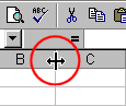
1. Place the cursor on the line between the B and C column headings. The cursor should look like the one displayed here, with two arrows.

2. Move your mouse to the right while holding down the left mouse button. The width indicator will appear on the screen.

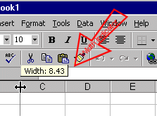
3. Release the left mouse button when the width indicator shows approximately 40.

In Microsoft Excel, each workbook is made up of several worksheets. Before moving to the next topic, move to a new worksheet.

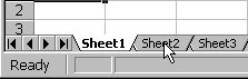
1. Click on Sheet2, which is located in the lower left corner of the screen.

Filling Cells Automatically

You can use Microsoft Excel to automatically fill cells with information that occur in a series. For example, you can have word automatically fill in times, the days of the week or months of the year, years, and other types of series. The following demonstrates:

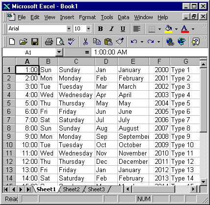
1. Type the following into the worksheet as shown.

2. Place the cursor in cell A1. 
3. Press F8. This will anchor the cursor.
4. Press the right arrow key six times to highlight cells A1 through G1.
5. Find the small black square in the lower right corner of the highlighted area. This is called the Fill Handle.

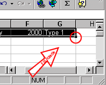
6. Grab the Fill Handle and drag with your mouse to highlight cells A1 to G24. 
7. Note how each cell fills.

2. Press Esc and then click anywhere on the worksheet to remove the highlighting.

This is the end of Lesson Two. Save your file and close Microsoft Excel.

1. Click on File, which is located on the Menu bar.
2. Press the down arrow key until Save is highlighted.
3. Press Enter.
4. Type lesson2.xls in the filename field.
5. Click on Save.
6. Click on File, which is located on the Menu bar.
7. Press the down arrow key until Exit is highlighted.
8. Press Enter.